Linear Regression Model

Predicting Sound Pressure in Wind Tunnel Using Linear Regression Model:

The main purpose of this project was to predict the sound pressure in an anechoic wind tunnel. This was done using data from the Airfoil Self-Noise Data Set in the following UCI Machine Learning Repository: link The rows of these files represent the data samples, while columns 1-5 are the features and the sound pressure output is column 6, as described below:

1. Frequency, in Hertz
2. Angle of attack, in degrees
3. Chord length, in meters
4. Free-stream velocity, in meters per second
5. Suction side displacement thickness, in meters
6. Scaled sound pressure level, in decibels

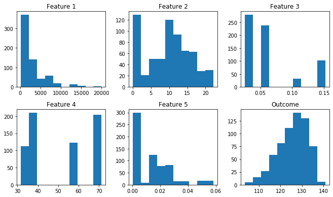
Data exploration: To begin, I first plotted a histogram of each feature and the output to see how they are distributed. What I found was that feature 1 is distributed mostly around 0-5000 Hertz, feature 2 is a little more evenly distributed, with the highestest distributions around 0-1 degrees and 10 degrees. Features 3 and 4 are distributed in 4 specific values, the rest of the values having no samples and feature 5 has the most samples between 0 and 0.01 meters. The outcome distribution increases until it peaks at around 128 decibels and then it decreases.

# read in training data
training_data = read_csv("airfoil_self_noise_train.csv")

# plot the histogram of each feature and outcome
fig, ax = plt.subplots(2,3)
fig.set_size_inches(9.25, 5.5)

ind = 0 
for i in range(2):
    for j in range(3):
        f1 = training_data.iloc[:,ind]
        ax[i][j].hist(f1)
        if (ind + 1) == 6:
            ax[i][j].set_title("Outcome")
        else:
            ax[i][j].set_title("Feature " + str(ind + 1))
        ind = ind + 1
plt.tight_layout()

Implementing a Linear Regression Model: After that, I implemented a linear regression model using the ordinary least squares (OLS) solution. In order to use this OLS formula, $w^{∗} = (X^{T} X)^{−1}X^{T} y$, I built a data matrix whose rows corresponded to the training samples and whose columns corresponded to the features (including the constant 1 for the intercept). I also defined a function to calculate the OLS using the formula as reference.

# function for ordinary least squares (OLS)
# 1) get transpose of X
# 2) calculate first half of equation: the inverse of the 
#    dot product of X transpose and X
# 3) calculate the second half of the equation: the dot 
#    product of X transpose and y

def OLS(X, y):
    transpose_X = X.transpose()
    first_half = np.linalg.inv(np.dot(transpose_X, X))
    second_half = np.dot(transpose_X, y)
    return np.dot(first_half, second_half)

# create dataframe for outcome values 
# y
outcomes = DataFrame(training_data.iloc[:,5])

# add column of 1's and remove the outcome column
# X
training_data.insert(0, "constant", [1] * len(training_data.iloc[:,1]), True)
training_data.drop('outcome', axis=1, inplace=True)

# use OLS to get weights
calculated_weights = OLS(training_data, outcomes)
calculated_weights

array([[ 1.32303685e+02],
       [-7.11322380e-04],
       [-4.54774159e-01],
       [-5.23017057e+01],
       [ 8.39826774e-02],
       [-9.14287813e+01]])

The liner regression model using the ordinary least squares solution has 6 parameters in this case.

After calculating the OLS solution, I tested the model on the test data and computed the residual sum of squares error (RSS) between the actual and predicted outcome variable. I ended up getting an RSS value of about 72.

# function to calculate the residual sum or squares error (RSS) 
# between the actual and predicted outcome
# 1) calculate the dot product of X and weights
# 2) calculate first half of equation: the transpose of the actual 
#    outcomes minus the dot product of X and the weights
# 3) calculate second half of equation: the actual outcomes minus 
#    the dot product of X and the weights
# 4) get the square root of the dot product of the first and second 
#    half of the equation

def RSS(X, w, y):
    x_dot_w = np.dot(X, w)
    first = (y - x_dot_w).transpose()
    second = y - x_dot_w
    return sqrt(np.dot(first, second))

# read in testing data
test_data = read_csv("airfoil_self_noise_test.csv")

# create dataframe for outcome values 
# y
test_outcomes = DataFrame(test_data.iloc[:,5])

# add column of 1's and remove the outcome column
# X
test_data.insert(0, "constant", [1] * len(test_data.iloc[:,1]), True)
test_data.drop('outcome', axis=1, inplace=True)

# calculate RSS
rss = RSS(test_data, calculated_weights, test_outcomes)
rss

71.66865682786033

We could stop there, but I decided to experiment with a few different feature combinations instead of using all of them to see if I could get a lower RSS value. You can see the results of this below, Using features 3 and 4 I got an RSS of about 133, using features 1, 2, and 5 I got an RSS of about 107 and when using features 1 and 4 I got an RSS of about 85.

# using features 3 and 4 
# remove other features from training data
training_data_f34 = training_data.drop(['f1', 'f2', 'f5'], axis=1, inplace=False)

# OLS for weights
calculated_weights_f34 = OLS(training_data_f34, outcomes)
print("weights:\n", calculated_weights_f34)

# remove other features from test data
test_data_f34 = test_data.drop(['f1','f2','f5'], axis=1, inplace=False)

# calculate RSS
rss = RSS(test_data_f34, calculated_weights_f34, test_outcomes)
print("\nRSS:", rss)

weights:
 [[ 1.25761164e+02]
 [-5.44150127e+01]
 [ 6.06585582e-02]]

RSS: 133.45352324493342

# using features 1, 2 and 5
# remove other features from training data
training_data_f125 = training_data.drop(['f3', 'f4'], axis=1, inplace=False)

# OLS for weights
calculated_weights_f125 = OLS(training_data_f125, outcomes)
print("weights:\n", calculated_weights_f125)

# remove other features from test data
test_data_f125 = test_data.drop(['f3','f4'], axis=1, inplace=False)

# calculate RSS
rss = RSS(test_data_f125, calculated_weights_f125, test_outcomes)
print("\nRSS:", rss)

weights:
 [[ 1.32516436e+02]
 [-5.76514811e-04]
 [-1.46030326e-01]
 [-2.60904487e+02]]

RSS: 107.44085921265567

# using features 1 and 4
# remove other features from training data
training_data_f14 = training_data.drop(['f2', 'f3', 'f5'], axis=1, inplace=False)

# OLS for weights
calculated_weights_f14 = OLS(training_data_f14, outcomes)
print("weights:\n", calculated_weights_f14)

# remove other features from test data
test_data_f14 = test_data.drop(['f2', 'f3', 'f5'], axis=1, inplace=False)

# calculate RSS
rss = RSS(test_data_f14, calculated_weights_f14, test_outcomes)
print("\nRSS:", rss)

weights:
 [[ 1.23150041e+02]
 [-1.39844979e-04]
 [ 5.75414946e-02]]

RSS: 85.24503305195404

While I wasn’t able to get and RSS value smaller than when I used all the features, I did not test all possible combinations, therefore, it might be possible to achieve a smaller RSS value with a different combination of features. The best way to go about this would probably be to write a program that goes through every possible feature combination and outputs the one with the lowest RSS value, the result from that would be the feature combination that would be the most useful to use when making predictions.