K-NN Classifier

Classifying Benign vs Malignant Tumors Using K-NN Classifier

The main purpose of this project was to classify whether a tumor is benign or malign based on its attributes. This was done using data from the following UCI Machine Learning Repository: link The rows of these files represent the data samples, while columns 1-9 are the features and the class variable is column 10, as described below:

1. Clump Thickness: discrete values {1, 10}
2. Uniformity of Cell Size: discrete values {1, 10}
3. Uniformity of Cell Shape: discrete values {1, 10}
4. Marginal Adhesion: discrete values {1, 10}
5. Single Epithelial Cell Size: discrete values {1, 10}
6. Bare Nuclei: discrete values {1, 10}
7. Bland Chromatin: discrete values {1, 10}
8. Normal Nucleoli: discrete values {1, 10}
9. Mitoses: discrete values {1, 10}
10. Class: 2 for benign, 4 for malignant

# import data from .csv file into table
training_data = Table.read_table('hw1_question1_train.csv')
training_data

f1	f2	f3	f4	f5	f6	f7	f8	f9	label
10	10	9	3	7	5	3	5	1	4
1	1	1	1	1	1	3	1	1	2
1	1	1	1	1	1	3	1	1	2
5	1	1	1	1	1	3	1	1	2
8	10	10	10	5	10	8	10	6	4
8	10	8	8	4	8	7	7	1	4
1	1	1	1	2	1	3	1	1	2
10	10	10	10	7	10	7	10	4	4
10	10	10	10	3	10	10	6	1	4
8	7	8	7	5	5	5	10	2	4

... (473 rows omitted)

Data exploration: First, I used the training data to count how many samples were in the benign and malignant classes. After doing this it’s clear that the samples are not evenly distributed and that there’s roughly a 1/3 ratio of malignant to benign tumors. This means there is a slightly higher chance of a tumor being benign than it being malignant.

# count the total number of samples in the benign/malignant class 
num_benign = training_data.where('label', are.equal_to(2)).num_rows
num_malignant = training_data.where('label', are.equal_to(4)).num_rows

print('Number of samples belonging to benign class:', num_benign) 
print('Number of samples belonging to malignant class:', num_malignant) 

Number of samples belonging to benign class: 330
Number of samples belonging to malignant class: 153

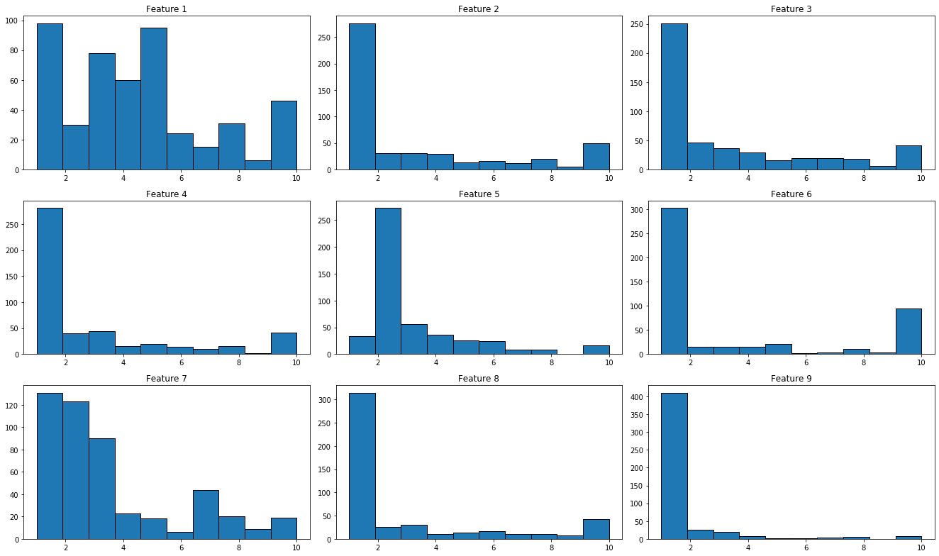
Next, I plotted a histogram of each feature using the training data to see how they are distributed in the 1-10 range among the samples. (i.e., 9 total histograms). From this, you can see that the features are not distributed evenly in the 1-10 range. Feature 1 is the most evenly distributed, however the majority of the samples are still equal to or less than five. Overall, the samples seem to have a higher distribution on the lower numbers.

For the next step, I randomly select 5 pairs of features and plotted them on scatter plots. Each data point is color-coded to indicate the class in which the samples belong to (e.g., blue for benign, red for malignant). Looking at the results from this graph, the data appears to be seperable, with the benign samples being concentrated on the bottom left of the graphs and the malignant samples being centered on the top right of the graphs.

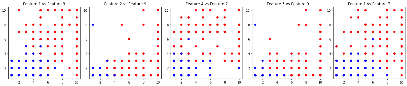
Implementing a K-Nearest Neighbor Classifier: Since the data does appear to seperable, K-NN is a valid model to use. If the data were not seperable into two groups, then K-NN would not be as good of a model for the data and would have a low classification accuracy. Now, to actually implement K-NN. In this project, I didn’t use any available libraries, instead I implemented the algorithm from scratch to better understand how it works. I also used two different distance metrics, the euclidean distance (l2-norm) and cosine similarity as distance measures to classify between the benign and malignant classes to see the difference in results.

###################### function definitions ######################
# calculates Euclidean distance (ED) btw two arrays of data

# the Euclidean distance is calculated by taking the square root
# of the sum of the squared differences of the arrays

# input: two arrays of numbers, arrays are same length

# output: returns the ED btw the two arrays of numbers 

def euclideanDistance(row1, row2):
    rows = np.subtract(row1,row2)
    distance = np.linalg.norm(rows)
    return distance 
    
# function to calculate cosine similarity for bonus

# input: two arrays of numbers, same length

# output: returns the cosine similarity between the two arrays

def cosineSimilarity(row1, row2):
    dot_prod = np.dot(row1, row2)
    norm1 = np.linalg.norm(row1)
    norm2 = np.linalg.norm(row2)
    denom = norm1 * norm2
    return dot_prod / denom


# function to get the K-Nearest Neighbors (k) in a set of arrays 
# (training_set) to one specific array (test_sample) by 
#     1) findining the Euclidean distance between each sample in 
#        the training_set and the test_sample and putting
#        them in a list called distances along with the
#        index of the corresponding row in the training_set
#     2) sort the list based on the distances (shortest to longest)
#     3) get the first k values from the distances list and return 
#        them in a list of tuples called neighbors 

# input: 1) an array of features of a sample who you want to find k 
#        neighbors for (test_sample)
#        2) a set of arrays of features for multiple samples who you 
#           will calculate the distance for against the testing 
#           array (training_set)
#        3) a value for k that will determine the number of closest 
#           samples that are returned

# output: a list of tuples of length k tha contains the row indexes 
#         in training arrays that are closest to the testing 
#         sample and the distance 

def getNeighbors(training_set, test_sample, k, dist_type):
    distances = []
    for i in range(training_set.num_rows):
        if dist_type == 'euclidean':
            d = euclideanDistance(training_set.row(i), test_sample)
        elif dist_type == 'cosine':
            d = cosineSimilarity(training_set.row(i), test_sample)
        elif dist_type == 'l0_norm':
            d = L0Norm(training_set.row(i), test_sample)
        distances.append((i, d))
    distances.sort(key=itemgetter(1))
    neighbors = []
    for i in range(k):
        neighbors.append(distances[i][0])
    return neighbors


# function to decide whether a sample belongs to class benign or 
# malignant based on its K-Nearest Neighbors by getting the label 
# of each neighbor, counting how many are benign and how many are 
# malignant and then returning whichever of the two classes had 
# the most votes

# input: list of tuples that has, index of row of neighbor and the 
# distance between the neighbor and sample we are trying to classify

# output: predicted label (either 2 or 4) of unlabeled sample

def getPredClass(neighbors):
    benign = 0
    malignant = 0
    for i in neighbors:
        if training_data.row(i)[9] == 4:
            malignant += 1
        else:
            benign += 1
    if benign > malignant:
        return 2
    else:
        return 4

For the next step, we want to figure out how well the K-NN model actually works on this dataset, so I wrote two functions to calculate both the accuracy and balanced accuracy of the model on the development set.

In addition to this, I explored the results with different values of k to see which resulted in better classification accuracies.

###################### function definitions ######################
# function to calculate the classification accuracy of the model, 
# accuracy is calculated as the number of correct classifications 
# over the total number of samples attempted to classify 

#input: array of actual label values and array of predicted label 
#       values

#output: accuracy of model

def getAcc(actual, pred):
    correct = 0
    for i in range(len(actual)):
        if actual[i] == pred[i]:
            correct += 1
    acc = (correct/(len(actual))) 
    return acc


# function to calculate the balanced classification accuracy of 
# the model, this is calculated as the number of correct 
# classifications of the first class over the total number of 
# samples in the first class summed by the number of classifications 
# of the second class ove the total number of samples in the second 
# class all divided by 2

#input: array of actual label values and array of predicted label 
#       values

#output: balanced accuracy of model

def getBalancedAcc(actual, pred):
    total_benign = np.count_nonzero(actual_label == 2)
    total_malignant = np.count_nonzero(actual_label == 4)
    correct_benign = 0
    correct_malignant = 0
    for i in range(len(actual)):
        if actual[i] == pred[i] and actual[i] == 2:
            correct_benign += 1
        elif actual[i] == pred[i] and actual[i] == 4:
            correct_malignant += 1
    bal_acc = ((correct_benign/total_benign) + (correct_malignant/total_malignant))/2
    return bal_acc

# setting up data for KNN abd Acc/BAcc calculations
no_labels_train = training_data.drop('label')            # remove labels from training data
labels_dev = Table().read_table('hw1_question2_dev.csv') # import dev data
no_labels_dev = labels_dev.drop('label')                 # remove labels from dev data
actual_label = labels_dev.column('label')                # put all dev data labels in array for Acc/BAcc check

# set up empty list to store values to put in table later
k_value = []
Acc_list = []
BAcc_list = []

# train model for values K = 1, 3, 5, 7, . . . , 19 using the train data
for k in range(1,20,2):
    predictions = []
    k_value.append(k)
    for i in range(no_labels_dev.num_rows):
        knn = getNeighbors(no_labels_train, no_labels_dev.row(i), k, 'euclidean')
        pred = getPredClass(knn)
        predictions.append(pred)
    # compute Acc and BAcc of model on dev set 
    Acc_list.append(getAcc(actual_label, predictions))
    BAcc_list.append(getBalancedAcc(actual_label, predictions))

    
# create table with all k-values and their corresponding Acc and BAcc values
model_test = Table().with_columns(
    'k-values', k_value,
    'Acc', Acc_list,
    'BAcc', BAcc_list)
model_test

k-values	Acc	BAcc
1	0.97	0.970856
3	0.99	0.991525
5	0.98	0.97933
7	0.97	0.967135
9	0.97	0.967135
11	0.97	0.967135
13	0.97	0.967135
15	0.97	0.967135
17	0.97	0.967135
19	0.97	0.967135

# plot the two metrics (Acc/BAcc) against the different values of K. 
model_test.plot('k-values')

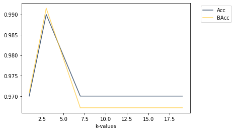
According to the graph above, which plots the accuracy and balanced accuracy against the different values of k, the best hyper-parameter k based on the accuracy metric is 3 and the best hyper-parameter k based on the balanced accuracy is also 3. In this case, the best hyper-parameters are the same k value.

Next, I tested the model on the test set using the best hyper-parameters found previously and calculated the accuracy and balanced accuracy based on these k-values.

# setting up data for KNN
labels_test = Table().read_table('hw1_question2_test.csv') # import test data
no_labels_test = labels_test.drop('label')                 # remove labels from test data

# running KNN on data
predictions = []
for i in range(no_labels_test.num_rows):
    knn = getNeighbors(no_labels_train, no_labels_test.row(i), 3, 'euclidean')
    pred = getPredClass(knn)
    predictions.append(pred)
    
# getting accuracies 
actual_label = labels_test.column('label')
print("Model Accuracy: ", getAcc(actual_label, predictions))
print("Model Balanced Accuracy: ", getBalancedAcc(actual_label, predictions))

Model Accuracy:  0.95
Model Balanced Accuracy:  0.9324324324324325

The accuracies calculated on the test set are lower than the ones calculated on the development set, which is understandable and could be explained by the data in the development set being more similar to the data in the training set than the testing set data.

For the above steps, I’d been using the Euclidean distance, so I then used cosine similarity instead to see if the resulting accuracies were better or not.

# set up empty list to store values to put in table later
k_value = []
Acc_list = []
BAcc_list = []

# train model for values K = 1, 3, 5, 7, . . . , 19 using the train data
for k in range(1,20,2):
    predictions = []
    k_value.append(k)
    for i in range(no_labels_dev.num_rows):
        cos_sim = getNeighbors(no_labels_train, no_labels_dev.row(i), k, 'cosine')
        pred = getPredClass(cos_sim)
        predictions.append(pred)
    # compute Acc and BAcc of model on dev set 
    Acc_list.append(getAcc(actual_label, predictions))
    BAcc_list.append(getBalancedAcc(actual_label, predictions))

    
# create table with all k-values and their corresponding Acc and BAcc values
model_test = Table().with_columns(
    'k-values', k_value,
    'Acc', Acc_list,
    'BAcc', BAcc_list)
model_test

k-values	Acc	BAcc
1	0.61	0.489704
3	0.63	0.55577
5	0.61	0.551051
7	0.56	0.511369
9	0.6	0.537538
11	0.55	0.492278
13	0.55	0.503432
15	0.58	0.527242
17	0.58	0.527242
19	0.58	0.527242

# plot the two metrics (Acc/BAcc) against the different values of K. 
model_test.plot('k-values')

# running Cosine Similarity on data
predictions = []
for i in range(no_labels_test.num_rows):
    cos_sim = getNeighbors(no_labels_train, no_labels_test.row(i), 3, 'cosine')
    pred = getPredClass(cos_sim)
    predictions.append(pred)
    
# getting accuracies 
actual_label = labels_test.column('label')
print("Model Accuracy: ", getAcc(actual_label, predictions))
print("Model Balanced Accuracy: ", getBalancedAcc(actual_label, predictions))

Model Accuracy:  0.27
Model Balanced Accuracy:  0.2365937365937366

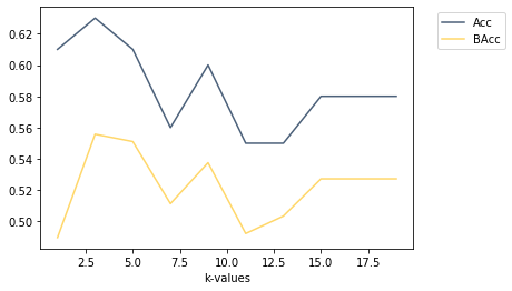
As you can see, using cosine similarity significanlty lowered the accuracies. The regular accuracy dropped from .93 to .27 and the balanced accuracy dropped from .93 to .24. This shows how important the distance metric used in K-NN is, as it can greatly determine whether the model is a good prediction model or not.